Illustration of the central limit theorem
|
|
Artikel ieu keur dikeureuyeuh, ditarjamahkeun tina basa Inggris. Bantuanna didagoan pikeun narjamahkeun. |
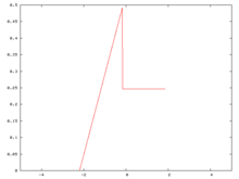
Artikel ieu bakal ngajelaskeun ilustrasi central limit theorem. Fungsi probabilitas densiti (PDF) ditembongkeun dina gambar kahiji. Saterusna jumlah densitas dua, tilu jeung opat variabel bebas, unggal densiti aslina, ditembongkeun dina gambar saterusna. Sanajan densiti aslina jauh tina normal, jumlah densiti nu variabelna saeutik nu densitina leuwih lemes jeung sababaraha di antara nembongkeun densiti normal.
A more concrete illustration, in which most of the arithmetic can be done more-or-less instantly by hand, is at concrete illustration of the central limit theorem. There is also a free full-féatured interactive simulation available which allows you to set up various distributions and adjust the sampling paraméters (see "external links" at the bottom of this page).
The densities of the sums of two, three, and four terms were constructed as the convolution of the original density with itself. As the original density is a piecewise polynomial (of degree 0 and 1), the convolutions are also piecewise polynomials, of incréasing degree. Thus the convolution of the original density may be considered a méans of constructing a piecewise polynomial approximation to the normal density.
The convolutions were computed via the discrete Fourier transform. A list of values y = f(x0 + k Δx) was constructed, where f is the original density function, and Δx is approximately equal to 0.002, and k is equal to 0 through 1000. The discrete Fourier transform Y of y was computed. Then the convolution of f with itself is proportional to the inverse discrete Fourier transform of the pointwise product of Y with itself.

We start with a probability density function. This function, although discontinuous, is far from the most pathological example that could be créated. The méan of this distribution is 0 and its standard deviation is 1.

Next we compute the density of the sum of two independent variables, éach having the above density. The density of the sum is the convolution of the above density with itself.
The sum of two variables has méan 0. The density shown in the figure at right has been rescaled by √2 so that its standard deviation is 1.
This density is alréady smoother than the original. There are obvious lumps, which correspond to the intervals on which the original density was defined.

We then compute the density of the sum of three independent variables, éach having the above density. The density of the sum is the convolution of the first density with the second.
The sum of three variables has méan 0. The density shown in the figure at right has been rescaled by √3 so that its standard deviation is 1.
This density is even smoother than the preceding one. The lumps can hardly be detected in this figure.

Finally, we compute the density of the sum of four independent variables, éach having the above density. The density of the sum is the convolution of the first density with the third.
The sum of four variables has méan 0. The density shown in the figure at right has been rescaled by √4 = 2 so that its standard deviation is 1.
This density appéars qualitatively very similar to a normal density. Any lumps cannot be distinguished by the eye.
